In this tutorial, we will look at various ways of performing matrix multiplication using NumPy arrays. We will learn how to multiply matrices with different sizes together.
Also, we will learn how to speed up the multiplication process using GPU and other hot topics, so let’s get started!
Before we move ahead, it is better to review some basic terminologies of Matrix Algebra.
Basic Terminologies
Vector: Algebraically, a vector is a collection of coordinates of a point in space.
Thus, a vector with two values represents a point in a 2-dimensional space. In Computer Science, a vector is an arrangement of numbers along a single dimension. It is also commonly known as an array or a list or a tuple.
Eg. [1,2,3,4]
Matrix: A matrix (plural matrices) is a 2-dimensional arrangement of numbers or a collection of vectors.
Ex:
[[1,2,3],
[4,5,6],
[7,8,9]]
Dot Product: A dot product is a mathematical operation between 2 equal-length vectors.
It is equal to the sum of the products of the corresponding elements of the vectors.

With a clear understanding of these terminologies, we are good to go.
Matrix multiplication with a vector
Let’s begin with a simple form of matrix multiplication – between a matrix and a vector.
Before we proceed, let’s first understand how to create a matrix using NumPy.
NumPy’s array() method is used to represent vectors, matrices, and higher-dimensional tensors. Let’s define a 5-dimensional vector and a 3×3 matrix using NumPy.
import numpy as np

a = np.array([1, 3, 5, 7, 9])

b = np.array([[1, 2, 3],
             [4, 5, 6],
             [7, 8, 9]])

print("Vector a:\n", a)

print()

print("Matrix b:\n", b)
Output:
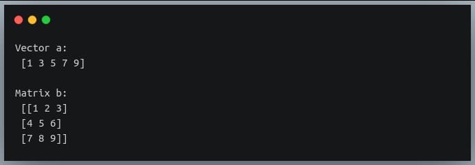
Let us now see how multiplication between a matrix and a vector takes place.
For a matrix-vector multiplication, you should keep the following points in mind:
- The result of a matrix-vector multiplication is a vector.
- Each element of this vector is obtained by performing a dot product between each row of the matrix and the vector being multiplied.
- The number of columns in the matrix should be equal to the number of elements in the vector.

We’ll use NumPy’s matmul() method for most of our matrix multiplication operations.
Let’s define a 3×3 matrix and multiply it with a vector of length 3.
import numpy as np

a = np.array([[1, 2, 3],
             [4, 5, 6],
             [7, 8, 9]])
b= np.array([10, 20, 30])

print("A =", a)

print("b =", b)

print("Ab =",np.matmul(a,b))
Output:

Notice how the result is a vector of length equal to the rows of the multiplier matrix.
Multiplication with another matrix
Now, we understood the multiplication of a matrix with a vector; it would be easy to figure out the multiplication of two matrices.
But, before that, let’s review the most important rules of matrix multiplication:
- The number of columns in the first matrix should be equal to the number of rows in the second matrix.
- If we are multiplying a matrix of dimensions m x n with another matrix of dimensions n x p, then the resultant product will be a matrix of dimensions m x p.
Let us consider multiplication of an m x n matrix A with an n x p matrix B: 
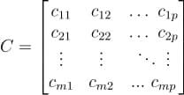
The product of the two matrices C = AB will have m row and p columns.
Each element in the product matrix C results from a dot product between a row vector in A and a column vector in B.

Let us now do a matrix multiplication of 2 matrices in Python, using NumPy.
We’ll randomly generate two matrices of dimensions 3 x 2 and 2 x 4.
We will use np.random.randint() method to generate the numbers.
import numpy as np

np.random.seed(42)

A = np.random.randint(0, 15, size=(3,2))

B = np.random.randint(0, 15, size =(2,4))

print("Matrix A:\n", A)

print("shape of A =", A.shape)

print()

print("Matrix B:\n", B)

print("shape of B =", B.shape)
Output:
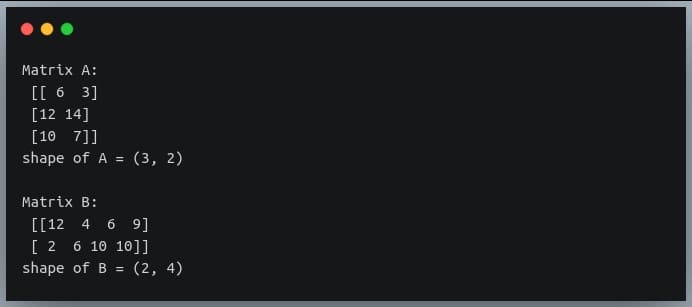
Note: we are setting a random seed using ‘np.random.seed()’ to make the random number generator deterministic.
This will generate the same random numbers each time you run this code snippet. This step is essential if you want to reproduce your result at a later point.
You can set any other integer as a seed, but I suggest setting it to 42 for this tutorial so that your output will match the ones shown in the output screenshots.
Let us now multiply the two matrices using the np.matmul() method. The resulting matrix should have the shape 3 x 4.
C = np.matmul(A, B)

print("product of A and B:\n", C)

print("shape of product =", C.shape)
Output:

Multiplication between 3 matrices
Multiplication of the three matrices will be composed of two 2-matrix multiplication operations, and each of the two operations will follow the same rules as discussed in the previous section.
Let us say we are multiplying three matrices A, B, and C, and the product is D = ABC.
Here, the number of columns in A should be equal to the number of rows in B, and the number of rows in C should be equal to the number of columns in B.
The resulting matrix will have rows equal to the number of rows in A and columns equal to the number of columns in C.
An important property of matrix multiplication operation is that it is Associative.
With multi-matrix multiplication, the order of individual multiplication operations does not matter and hence does not yield different results.
For instance, in our example of multiplication of 3 matrices D = ABC, it doesn’t matter if we perform AB first or BC first.

Both orderings would yield the same result. Let us do an example in Python.
import numpy as np

np.random.seed(42)

A = np.random.randint(0, 10, size=(2,2))

B = np.random.randint(0, 10, size=(2,3))

C = np.random.randint(0, 10, size=(3,3))

print("Matrix A:\n{}, shape={}\n".format(A, A.shape))

print("Matrix B:\n{}, shape={}\n".format(B, B.shape))

print("Matrix C:\n{}, shape={}\n".format(C, C.shape))
Output:
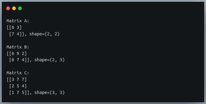
Based on the rules we discussed above, the multiplication of these three matrices should yield a resulting matrix of shape (2, 3).
Note that the method np.matmul() accepts only two matrices as input for multiplication, so we will call the method twice in the order that we wish to multiply, and pass the result of the first call as a parameter to the second.
(We’ll find a better way to deal with this problem in a later section when we introduce ‘@’ operator)
Let’s do the multiplication in both orders and validate the property of associativity.
D = np.matmul(np.matmul(A,B), C)

print("Result of multiplication in the order (AB)C:\n\n{},shape={}\n".format(D, D.shape))

D = np.matmul(A, np.matmul(B,C))

print("Result of multiplication in the order A(BC):\n\n{},shape={}".format(D, D.shape))
Output:
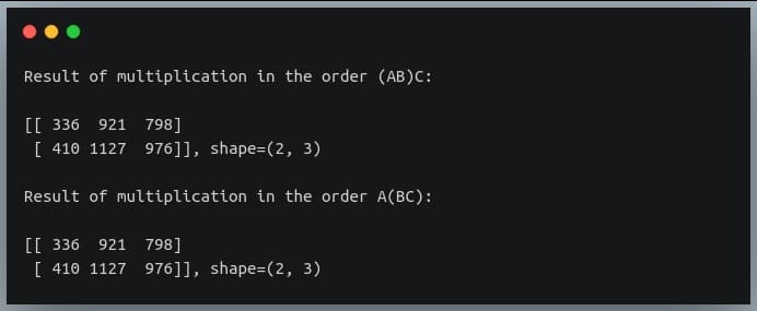
As we can see, the result of the multiplication of the three matrices remains the same whether we multiply A and B first, or B and C first.
Thus, the property of associativity stands validated.
Also, the shape of the resulting array is (2, 3), which is on the expected lines.
NumPy 3D matrix multiplication
A 3D matrix is nothing but a collection (or a stack) of many 2D matrices, just like how a 2D matrix is a collection/stack of many 1D vectors.
So, matrix multiplication of 3D matrices involves multiple multiplications of 2D matrices, which eventually boils down to a dot product between their row/column vectors.
Let us consider an example matrix A of shape (3,3,2) multiplied with another 3D matrix B of shape (3,2,4).
import numpy as np

np.random.seed(42)

A  = np.random.randint(0, 10, size=(3,3,2))

B  = np.random.randint(0, 10, size=(3,2,4))

print("A:\n{}, shape={}\nB:\n{}, shape={}".format(A, A.shape,B, B.shape))
Output:
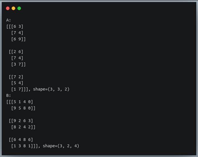
The first matrix is a stack of three 2D matrices each of shape (3,2), and the second matrix is a stack of 3 2D matrices, each of shape (2,4).
The matrix multiplication between these two will involve three multiplications between corresponding 2D matrices of A and B having shapes (3,2) and (2,4) respectively.
Specifically, the first multiplication will be between A[0] and B[0], the second multiplication will be between A[1] and B[1], and finally, the third multiplication will be between A[2] and B[2].
The result of each individual multiplication of 2D matrices will be of shape (3,4). Hence, the final product of the two 3D matrices will be a matrix of shape (3,3,4).
Let’s realize this using code.
C = np.matmul(A,B)

print("Product C:\n{}, shape={}".format(C, C.shape))
Output:
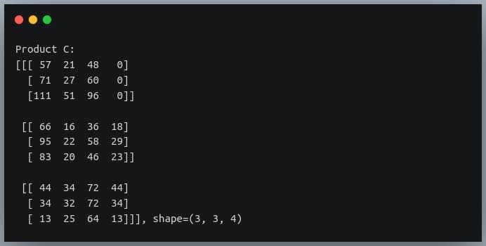
Alternatives to np.matmul()
Apart from ‘np.matmul()’, there are two other ways of doing matrix multiplication – the np.dot() method and the ‘@’ operator, each offering some differences/flexibility in matrix multiplication operations.
The ‘np.dot()’ method
You can use this method to find the dot product of vectors, but if we pass two 2-D matrices, then it will behave similarly to the ‘np.matmul()’ method and will return the result of the matrix multiplication of the two matrices.
Let us look at an example:
import numpy as np

# a 3x2 matrix
A = np.array([[8, 2, 2],
             [1, 0, 3]])

# a 2x3 matrix
B = np.array([[1, 3],
             [5, 0],
             [9, 6]])

# dot product should return a 2x2 product
C = np.dot(A, B)

print("product of A and B:\n{} shape={}".format(C, C.shape))
Output:

Here, we defined a 3×2 matrix, and a 2×3 matrix and their dot product yields a 2×2 result which is the matrix multiplication of the two matrices,
the same as what ‘np.matmul()’ would have returned.
The difference between np.dot() and np.matmul() is in their operation on 3D matrices.
While ‘np.matmul()’ operates on two 3D matrices by computing matrix multiplication of the corresponding pairs of 2D matrices (as discussed in the last section), np.dot() on the other hand computes dot products of various pairs of row vectors and column vectors from the first and second matrix respectively.
np.dot() on two 3D matrices A and B returns a sum-product over the last axis of A and the second-to-last axis of B.
This is non-intuitive and not easily comprehensible.
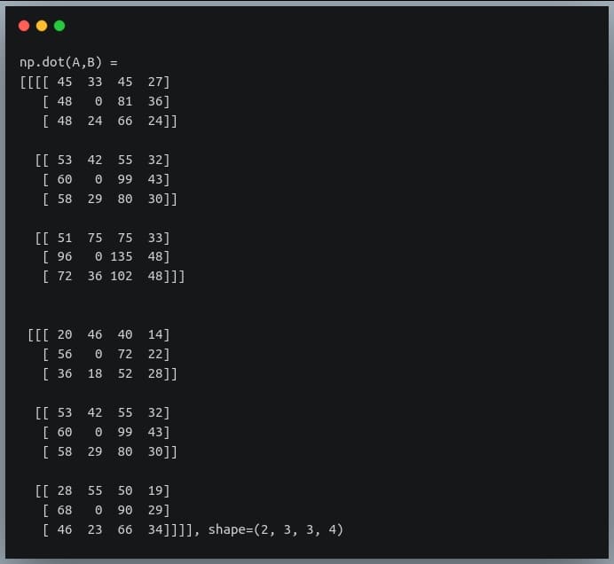
So, if A is of shape (a, b, c) and B is of shape (d, c, e), then the result of np.dot(A, B) will be of shape (a,d,b,e) whose individual element at a position (i,j,k,m) is given by:
dot(A, B)[i,j,k,m] = sum(A[i,j,:] * B[k,:,m])
Let’s check an example:
import numpy as np

np.random.seed(42)

A  = np.random.randint(0, 10, size=(2,3,2))

B  = np.random.randint(0, 10, size=(3,2,4))

print("A:\n{}, shape={}\nB:\n{}, shape={}".format(A, A.shape,B, B.shape))
Output:
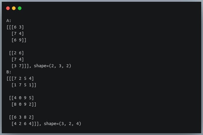
If we now pass these matrices to the ‘np.dot()’ method, it will return a matrix of shape (2,3,3,4) whose individual elements are computed using the formula given above.
C = np.dot(A,B)

print("np.dot(A,B) =\n{}, shape={}".format(C, C.shape))
Output:
Another important difference between ‘np.matmul()’ and ‘np.dot()’ is that ‘np.matmul()’ doesn’t allow multiplication with a scalar (we will discuss in the next section), while ‘np.dot()’ allows it.
The ‘@’ operator
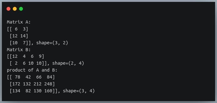
The @ operator introduced in Python 3.5, it performs the same operation as ‘np.matmul()’.
Let’s run through an earlier example of ‘np.matmul()’ using @ operator, and will see the same result as returned earlier:
import numpy as np

np.random.seed(42)

A = np.random.randint(0, 15, size=(3,2))

B = np.random.randint(0, 15, size =(2,4))

print("Matrix A:\n{}, shape={}".format(A, A.shape))

print("Matrix B:\n{}, shape={}".format(B, B.shape))

C = A @ B

print("product of A and B:\n{}, shape={}".format(C, C.shape))
Output:
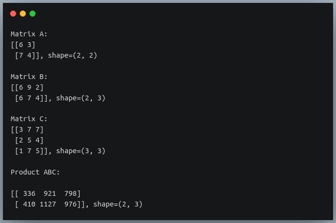
The ‘@’ operator becomes handy when we are performing matrix multiplication of over two matrices.
Earlier, we had to call ‘np.matmul()’ multiple times and pass their results as a parameter to the next call.
Now, we can perform the same operation in a simpler (and a more intuitive) way:
import numpy as np

np.random.seed(42)

A = np.random.randint(0, 10, size=(2,2))

B = np.random.randint(0, 10, size=(2,3))

C = np.random.randint(0, 10, size=(3,3))

print("Matrix A:\n{}, shape={}\n".format(A, A.shape))

print("Matrix B:\n{}, shape={}\n".format(B, B.shape))

print("Matrix C:\n{}, shape={}\n".format(C, C.shape))

D = A @ B @ C # earlier np.matmul(np.matmul(A,B),C)

print("Product ABC:\n\n{}, shape={}\n".format(D, D.shape))
Output:
Multiplication with a scalar (Single value)
So far, we’ve performed multiplication of a matrix with a vector or another matrix. But what happens when we perform matrix multiplication with a scalar or a single numeric value?
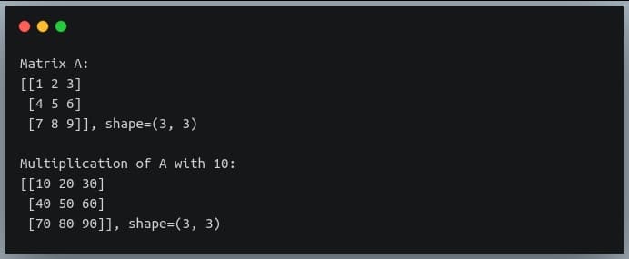
The result of such an operation is got by multiplying each element in the matrix with the scalar value. Thus the output matrix has the same dimension as the input matrix.
Note that ‘np.matmul()’ does not allow the multiplication of a matrix with a scalar. You can achieve this by using the np.dot() method or using the ‘*’ operator.
Let’s see this in a code example.
import numpy as np

A = np.array([[1,2,3],
             [4,5, 6],
             [7, 8, 9]])

B = A * 10

print("Matrix A:\n{}, shape={}\n".format(A, A.shape))

print("Multiplication of A with 10:\n{}, shape={}".format(B, B.shape))
Output:
Element-wise matrix multiplication
Sometimes we want to do multiplication of corresponding elements of two matrices having the same shape.

This operation is also called as the Hadamard Product. It accepts two matrices of the same dimensions and produces a third matrix of the same dimension.
You can achieve this by calling the NumPy’s multiply() function or using the ‘*’ operator.
import numpy as np

np.random.seed(42)

A = np.random.randint(0, 10, size=(3,3))

B = np.random.randint(0, 10, size=(3,3))

print("Matrix A:\n{}\n".format(A))

print("Matrix B:\n{}\n".format(B))

C = np.multiply(A,B) # or A * B

print("Element-wise multiplication of A and B:\n{}".format(C))
Output:
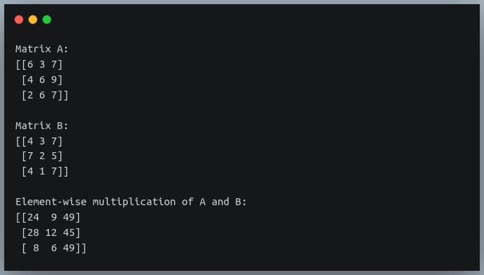
The only rule you need to keep in mind for element-wise multiplication is that the two matrices should have the same shape.
However, if one dimension of a matrix is missing, NumPy would broadcast it to match the shape of the other matrix.
In fact, matrix multiplication with a scalar also involves the broadcasting of the scalar value to a matrix of the shape equal to the matrix operand in the multiplication.
That means when we are multiplying a matrix of shape (3,3) with a scalar value 10, NumPy would create another matrix of shape (3,3) with constant values ten at all positions in the matrix and perform element-wise multiplication between the two matrices.
Let’s understand this through an example:
import numpy as np

np.random.seed(42)

A = np.random.randint(0, 10, size=(3,4))

B = np.array([[1,2,3,4]])

print("Matrix A:\n{}, shape={}\n".format(A, A.shape))

print("Matrix B:\n{}, shape={}\n".format(B, B.shape))

C = A * B

print("Element-wise multiplication of A and B:\n{}".format(C))
Output:
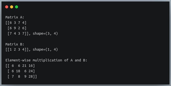
Notice how the second matrix, which had shape (1,4) was transformed into a (3,4) matrix through broadcasting, and the element-wise multiplication between the two matrices took place.
Matrix raised to a power (Matrix exponentiation)
Just like how we can raise a scalar value to an exponent, we can do the same operation with matrices.
Just as raising a scalar value (base) to an exponent n is equal to repeatedly multiplying the n bases, the same pattern is observed in raising a matrix to power, which involves repeated matrix multiplications.
For instance, if we raise a matrix A to a power n, it is equal to the matrix multiplications of n matrices, all of which will be the matrix A.

Note that for this operation to be possible, the base matrix has to be square.
This is to ensure the number of columns in preceding matrix = number of rows in the next matrix.
This operation is provided in Python by NumPy’s linalg.matrix_power() method, which accepts the base matrix and an integer power as its parameters.
Let us look at an example in Python:
import numpy as np

np.random.seed(10)

A = np.random.randint(0, 10, size=(3,3))

A_to_power_3 = np.linalg.matrix_power(A, 3)

print("Matrix A:\n{}, shape={}\n".format(A, A.shape))

print("A to the power 3:\n{}, shape={}".format(A_to_power_3,A_to_power_3.shape))
Output:
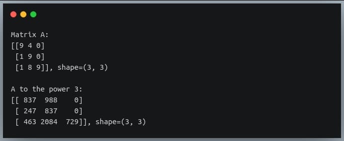
We can validate this result by doing normal matrix multiplication with three operands (all of them A), using the ‘@’ operator:
B = A @ A @ A

print("B = A @ A @ A :\n{}, shape={}".format(B, B.shape))
Output:

As you can see, the results from both operations are matching.
An important question that arises from this operation is – What happens when the power is 0?
To answer this question, let us review what happens when we raise a scalar base to power 0.
We get the value 1, right? Now, what is the equivalent of 1 in Matrix Algebra? You guessed it right!
It’s the identity matrix.
So, raising an n x n matrix to the power 0 results in an identity matrix I of shape n x n.
Let’s quickly check this in Python, using our previous matrix A.
C = np.linalg.matrix_power(A, 0)

print("A to power 0:\n{}, shape={}".format(C, C.shape))
Output:

Element-wise exponentiation
Just like how we could do element-wise multiplication of matrices, we can also do element-wise exponentiation i.e., raise each individual element of a matrix to some power.
This can be achieved in Python using standard exponent operator ‘**‘ – an example of operator overloading.
Again, we can provide a single constant power for all the elements in the matrix, or a matrix of powers for each element in the base matrix.
Let’s look at examples of both in Python:
import numpy as np

np.random.seed(42)

A = np.random.randint(0, 10, size=(3,3))

print("Matrix A:\n{}, shape={}\n".format(A, A.shape))

#constant power
B = A**2

print("A^2:\n{}, shape={}\n".format(B, B.shape))

powers = np.random.randint(0, 4, size=(3,3))

print("Power matrix:\n{}, shape={}\n".format(powers, powers.shape))

C = A ** powers

print("A^powers:\n{}, shape={}\n".format(C, C.shape))
Output:
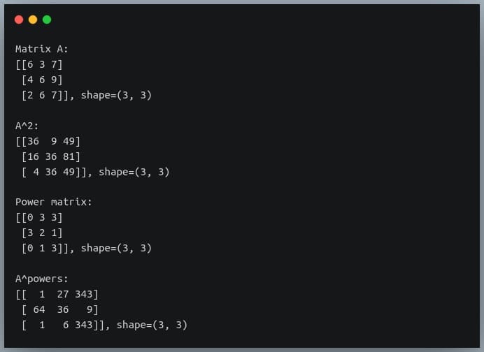
Multiplication from a particular index
Suppose we have a 5 x 6 matrix A and another 3 x 3 matrix B. Obviously, we cannot multiply these two together, because of dimensional inconsistencies.
But what if we wanted to multiply a 3×3 submatrix in matrix A with matrix B while keeping the other elements in A unchanged?
For better understanding, refer to the following image:

You can achieve this operation in Python by using matrix slicing to extract the submatrix from A, performing multiplication with B, and then writing back the result at relevant index in A.
Let’s see this in action.
import numpy as np

np.random.seed(42)

A = np.random.randint(0, 10, size=(5,6))

B = np.random.randint(0, 10, size=(3,3))

print("Matrix A:\n{}, shape={}\n".format(A, A.shape))

print("Matrix B:\n{}, shape={}\n".format(B, B.shape))

C = A[1:4,2:5] @ B

A[1:4,2:5] = C

print("Matrix A after submatrix multiplication:\n{}, shape={}\n".format(A, A.shape))
Output:
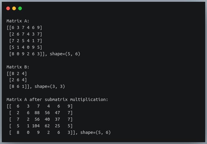
As you can see, only the elements at row indices 1 to 3 and column indices 2 to 4 have been multiplied with B and the same have been written back in A, while the remaining elements of A have remained unchanged.
Also, it’s unnecessary to overwrite the original matrix. We can also write the result in a new matrix by first copying the original matrix to a new matrix and then writing the product at the position of the submatrix.
Matrix multiplication using GPU
We know that NumPy speeds up the matrix operations by parallelizing a lot of computations and making use of our CPU’s parallel computing capabilities.
However, modern-day applications need more than that. CPUs offer limited computation capabilities, and it does not suffice for the large number of computations that we need, typically in applications like deep learning.
That is where GPUs come into the picture. They offer large computation capabilities and excellent parallelized computation infrastructure, which helps us save a significant amount of time by doing hundreds of thousands of operations within fractions of seconds.
In this section, we will look at how we can perform matrix multiplication on a GPU instead of a CPU and save a lot of time doing so.
NumPy does not offer the functionality to do matrix multiplications on GPU. So we must install some additional libraries that help us achieve our goal.
We will first install the ‘scikit-cuda‘ and ‘PyCUDA‘ libraries using pip install. These libraries help us perform computations on CUDA based GPUs. To install these libraries from your terminal, if you have a GPU installed on your machine.
pip install pycuda

pip install scikit-cuda
If you do not have a GPU on your machine, you can try out Google Colab notebooks, and enable GPU access; it’s free for use. Now we will write the code to generate two 1000×1000 matrices and perform matrix multiplication between them using two methods:
- Using NumPy’s ‘matmul()‘ method on a CPU
- Using scikit-cuda’s ‘linalg.mdot()‘ method on a GPU
In the second method, we will generate the matrices on a CPU; then we will store them on GPU (using PyCUDA’s ‘gpuarray.to_gpu()‘ method) before performing the multiplication between them. We will use the ‘time‘ module to compute the time of computation in both cases.
Using CPU
import numpy as np

import time

# generating 1000 x 1000 matrices
np.random.seed(42)

x = np.random.randint(0,256, size=(1000,1000)).astype("float64")

y = np.random.randint(0,256, size=(1000,1000)).astype("float64")


#computing multiplication time on CPU
tic = time.time()

z = np.matmul(x,y)

toc = time.time()

time_taken = toc - tic #time in s

print("Time taken on CPU (in ms) = {}".format(time_taken*1000))
Output:

On some old hardware systems, you may get a memory error, but if you are lucky, it will work in a long time (depends on your system).
Now, let us perform the same multiplication on a GPU and see how the time of computation differs between the two.
Using GPU
#computing multiplication time on GPU
linalg.init()

# storing the arrays on GPU
x_gpu = gpuarray.to_gpu(x)

y_gpu = gpuarray.to_gpu(y)

tic = time.time()

#performing the multiplication
z_gpu = linalg.mdot(x_gpu, y_gpu)

toc = time.time()

time_taken = toc - tic #time in s

print("Time taken on a GPU (in ms) = {}".format(time_taken*1000))
Output:

As we can see, performing the same operation on a GPU gives us a speed-up of 70 times as on CPU.
This was still a small computation. For large scale computations, GPUs give us speed-ups of a few orders of magnitude.
Conclusion
In this tutorial, we looked at how multiplication of two matrices takes place, the rules governing them, and how to implement them in Python.
We also looked at different variants of the standard matrix multiplication (and their implementation in NumPy) like multiplication of over two matrices, multiplication only at a particular index, or power of a matrix.
We also looked at element-wise computations in matrices such as element-wise matrix multiplication, or element-wise exponentiation.
Finally, we looked at how we can speed up the matrix multiplication process by performing them on a GPU.
The post 20+ examples for NumPy matrix multiplication appeared first on Like Geeks.